Sigma Rules and Measures of Central Location

📹 Video Overview

🎯 What We're Learning Today

Main Topics:

1. Sigma Rules (∑) - Math shortcuts for summations

2. Measures of Central Location - Finding the "middle" or "typical" value

   • Mode (most common)

   • Mean (average)

   • Median (middle value)

---

Part 1: Sigma Rules (∑)

🔤 What is Sigma (∑)?

Sigma (∑) = Mathematical shorthand for "add everything up"

Example: Defective items in 10 shipments: 3, 4, 1, 5, 2, 3, 2, 6, 3, 1

Instead of writing: x₁ + x₂ + x₃ + x₄ + x₅ + x₆ + x₇ + x₈ + x₉ + x₁₀

We write:

$\sum_{i=1}^{n} x_i$

💡 Memory hack: Think of ∑ as a "smart calculator" that knows to add everything from position 1 to n.

Breaking down the notation:

  n          ← Stop here (n = 10 in our example)
  ∑ x_i      ← Sum all x values
 i=1         ← Start here (first observation)

---

📐 The 5 Essential Sigma Rules

Rule 1: Sum of a Constant

Formula:

$\sum_{i=1}^{n} a = n \times a$

Plain English: If you add the same number n times, just multiply!

Example: Data series: 3, 3, 3, 3, 3 (n = 5)

$\sum_{i=1}^{5} 3 = 3 + 3 + 3 + 3 + 3 = 5 \times 3 = 15$

💡 Memory hack: Adding 5 threes is just 5 × 3. Don't overthink it!

---

Rule 2: Sum of a Constant × Variable

Formula:

$\sum_{i=1}^{n} a \times x_i = a \times \sum_{i=1}^{n} x_i$

Plain English: You can "pull out" the constant from the sum!

Example: Defective items: 3, 4, 1, 5, 2, 3, 2, 6, 3, 1

If each defective item costs 5 NIS (a = 5), what's the total damage?

$\sum_{i=1}^{10} 5x_i = 5 \times \sum_{i=1}^{10} x_i = 5 \times (3+4+1+5+2+3+2+6+3+1) = 5 \times 30 = 150 \text{ NIS}$

💡 Memory hack: The constant is like a "multiplier hat" - you can put it on at the end instead of on each item!

---

Rule 3: Sum of Addition

Formula:

$\sum_{i=1}^{n} (x_i + y_i) = \sum_{i=1}^{n} x_i + \sum_{i=1}^{n} y_i$

Plain English: Sum of sums = sum of each separately!

Example:

xᵢ	yᵢ	xᵢ + yᵢ
1	3	4
2	4	6
3	6	9

$\sum_{i=1}^{3} (x_i + y_i) = 4 + 6 + 9 = 19$

OR:

$\sum_{i=1}^{3} x_i + \sum_{i=1}^{3} y_i = (1+2+3) + (3+4+6) = 6 + 13 = 19$

💡 Memory hack: Addition is "friendly" - you can split it up!

---

Rule 4: Sum of Multiplication (TRICKY!)

Formula:

$\sum_{i=1}^{n} (x_i \times y_i) \neq \sum_{i=1}^{n} x_i \times \sum_{i=1}^{n} y_i$

Plain English: You CANNOT split multiplication! Must multiply first, then sum.

Example:

xᵢ	yᵢ	xᵢ × yᵢ
1	3	3
2	4	8
3	6	18

CORRECT:

$\sum_{i=1}^{3} (x_i \times y_i) = 3 + 8 + 18 = 29$

WRONG:

$\sum_{i=1}^{3} x_i \times \sum_{i=1}^{3} y_i = 6 \times 13 = 78 \neq 29$

⚠️ CRITICAL: Multiplication is NOT friendly! Don't split it!

💡 Memory hack: "Multiply INSIDE the sum, not outside!"

---

Rule 5: Sum of Squares (ALSO TRICKY!)

Formula:

$\sum_{i=1}^{n} x_i^2 \neq \left(\sum_{i=1}^{n} x_i\right)^2$

Plain English: Square each value first, THEN sum. Not the other way around!

Example:

xᵢ	xᵢ²
1	1
2	4
3	9

CORRECT:

$\sum_{i=1}^{3} x_i^2 = 1 + 4 + 9 = 14$

WRONG:

$\left(\sum_{i=1}^{3} x_i\right)^2 = (1+2+3)^2 = 6^2 = 36 \neq 14$

⚠️ CRITICAL: Square INSIDE first, then add!

💡 Memory hack: "Square the individuals, not the team!"

---

📋 Sigma Rules Quick Reference

---

🧮 Practice Problem: Complete Walkthrough

Given:

xᵢ	yᵢ
1	3
2	4
3	6

Problem 1: Calculate $\sum_{i=1}^{3} (2x_i + 3y_i)$

Solution:

$\sum_{i=1}^{3} (2x_i + 3y_i) = \sum_{i=1}^{3} 2x_i + \sum_{i=1}^{3} 3y_i$

$= 2\sum_{i=1}^{3} x_i + 3\sum_{i=1}^{3} y_i$

$= 2(1+2+3) + 3(3+4+6)$

$= 2(6) + 3(13) = 12 + 39 = 51$

---

Problem 2: Calculate $\sum_{i=1}^{3} (x_i + y_i)^2$

Solution:

First expand: $(x_i + y_i)^2 = x_i^2 + 2x_iy_i + y_i^2$

$\sum_{i=1}^{3} (x_i + y_i)^2 = \sum_{i=1}^{3} x_i^2 + 2\sum_{i=1}^{3} x_iy_i + \sum_{i=1}^{3} y_i^2$

Calculate each part:

• $\sum x_i^2 = 1^2 + 2^2 + 3^2 = 1 + 4 + 9 = 14$

• $\sum x_iy_i = (1×3) + (2×4) + (3×6) = 3 + 8 + 18 = 29$

• $\sum y_i^2 = 3^2 + 4^2 + 6^2 = 9 + 16 + 36 = 61$

Final answer:

$14 + 2(29) + 61 = 14 + 58 + 61 = 133$

---

Part 2: Measures of Central Location

🎯 The Big Question

What's a "typical" or "representative" value in the data?

Example claim: "Economists earn more than teachers"

Does EVERY economist earn more than EVERY teacher? No!

So we need a way to describe the "center" of the data.

Three main measures:

---

📊 Measure 1: Mode (x̂)

Definition: The value (or category) that appears MOST frequently

Notation: x̂ (x-hat)

For Qualitative Variables:

Example: Preferred social network

Social Network	f(x)
Instagram	43
Facebook	16
Twitter	4
TikTok	2
LinkedIn	1
None	7

Mode = Instagram (highest frequency)

💡 Memory hack: Mode = Most popular = Most Often Displayed Everywhere

---

For Discrete Quantitative Variables:

Example: Number of people in family

People (x)	f(x)
2	3
3	2
4	1
5	3
6	1

Mode = 2 and 5 (both appear 3 times - bimodal!)

---

For Continuous Quantitative Variables:

Example: Test scores

Scores	f(x)	l	d
40-60	5	20	0.25
60-70	5	10	0.5
70-75	10	5	2
75-85	10	10	1
85-100	15	15	1

Mode = 72.5 (middle of class 70-75, which has highest density d = 2)

⚠️ Important: For continuous variables, use DENSITY (d), not frequency!

💡 Memory hack: The modal class is the "densest crowd"

---

🔍 Characteristics of Mode:

✓ Not affected by extreme values

✓ Not affected by other frequencies (only cares about the winner)

✗ Can have multiple modes (bimodal, multimodal)

✗ Might not represent the "center" well

---

📊 Measure 2: Mean (x̄)

Definition: The arithmetic average - sum all values and divide by count

Notation: x̄ (x-bar)

Basic Formula:

$\bar{x} = \frac{\sum_{i=1}^{n} x_i}{n} = \frac{x_1 + x_2 + ... + x_n}{n}$

Example: Number of people in family: 2, 2, 6, 5, 3, 5, 5, 4, 3, 2

$\bar{x} = \frac{2+2+6+5+3+5+5+4+3+2}{10} = \frac{37}{10} = 3.7$

💡 Memory hack: Mean = What everyone would get if we distributed equally

---

Mean from Frequency Table:

Formula:

$\bar{x} = \frac{\sum_{i=1}^{k} x_i \times f_i}{\sum_{i=1}^{k} f_i} = \sum_{i=1}^{k} x_i \times p_i$

Why? If 2 appears 3 times, instead of writing 2+2+2, write 2×3!

Example:

x	f(x)	p(x)	x × f(x)	x × p(x)
2	3	30%	6	0.6
3	2	20%	6	0.6
4	1	10%	4	0.4
5	3	30%	15	1.5
6	1	10%	6	0.6
Total	10	100%	37	3.7

Using frequencies:

$\bar{x} = \frac{37}{10} = 3.7$

Using relative frequencies:

$\bar{x} = 0.6 + 0.6 + 0.4 + 1.5 + 0.6 = 3.7$

💡 Memory hack: "Multiply before you divide" - weight each value by how often it appears!

---

Mean for Continuous Variables:

Use the MIDPOINT of each class!

Example: Test scores

Scores	f(x)	Midpoint (xᵢ)	xᵢ × f(x)
40-60	5	50	250
60-70	5	65	325
70-75	10	72.5	725
75-85	10	80	800
85-100	10	92.5	925
Total	40	-	3025

$\bar{x} = \frac{3025}{40} = 75.625$

How to find midpoint:

$\text{Midpoint} = \frac{\text{Lower limit} + \text{Upper limit}}{2}$

Example: For 40-60 → Midpoint = (40+60)/2 = 50

---

🔍 Characteristics of Mean:

✓ Uses all data - every value matters

✓ Most common measure - used everywhere

✗ Affected by extreme values (outliers can pull it way off!)

✗ May not be an actual data value (can't have 3.7 people!)

Special Property: Sum of deviations from mean = 0

$\sum_{i=1}^{n} (x_i - \bar{x}) = 0$

Example: Data: 2, 2, 6, 5, 3, 5, 5, 4, 3, 2 (x̄ = 3.7)

xᵢ	xᵢ - x̄
2	-1.7
2	-1.7
6	+2.3
5	+1.3
3	-0.7
5	+1.3
5	+1.3
4	+0.3
3	-0.7
2	-1.7

Sum = 0 ✓

💡 Memory hack: The mean is like a "balance point" - negatives and positives cancel out!

---

📊 Measure 3: Median (x̃)

Definition: The middle value when data is sorted - splits data 50-50

Notation: x̃ (x-tilde)

How to Find Median:

Step 1: Sort data from smallest to largest

Step 2: Find the middle position

---

If n is ODD:

Formula:

$\tilde{x} = x_{\frac{n+1}{2}}$

Example: Scores: 50, 60, 60, 70, 80 (n = 5)

Position of median = (5+1)/2 = 3rd value

Median = 60

---

If n is EVEN:

Formula:

$\tilde{x} = \frac{x_{\frac{n}{2}} + x_{\frac{n}{2}+1}}{2}$

Example: Scores: 50, 60, 60, 70, 80, 90 (n = 6)

Positions: 6/2 = 3rd and 4th values

Median = (60 + 70)/2 = 65

💡 Memory hack:

• Odd: One clear middle person

• Even: Two middle people, average them!

---

Median from Frequency Table:

Example: Number of people in family (n = 20)

x	f(x)	F(x)
2	3	3
3	5	8
4	6	14
5	3	17
6	3	20

Find: Position n/2 = 20/2 = 10th value

Look at F(x):

• F(4) = 14 (14 observations up to x=4)

• F(3) = 8 (8 observations up to x=3)

The 10th value is in the x=4 category!

Median = (x₁₀ + x₁₁)/2 = (4 + 4)/2 = 4

---

Median for Continuous Variables:

Find the "median class" - the class containing position n/2

Example: Test scores (n = 100)

Scores	f(x)	F(x)
40-60	5	5
60-70	10	15
70-75	20	35
75-85	40	75
85-100	25	100

Position n/2 = 100/2 = 50th value

• F(70-75) = 35 (not enough)

• F(75-85) = 75 (includes position 50!)

Median is in class 75-85

💡 Memory hack: Keep adding F(x) until you pass n/2!

---

🔍 Characteristics of Median:

✓ Not affected by extreme values (only cares about position, not actual values!)

✓ Always an actual possible value (for discrete) or in a real class

✗ Doesn't use information from all values

Powerful example:

Salaries: 3000, 4000, 4700, 5000, 5500

Median = 4700 (middle value)

Now change 5500 to 5,500,000!

Median still = 4700 (position unchanged!)

Mean would jump dramatically!

💡 Memory hack: Median is the "bodyguard" - protects against extreme outliers!

---

🔄 Linear Transformations

What if we add/multiply all values by a constant?

Rules:

If $z_i = a + bx_i$ (where a and b are constants):

$\bar{z} = a + b\bar{x}$

$\tilde{z} = a + b\tilde{x}$

$\hat{z} = a + b\hat{x}$

Example: Test scores of 7 students: 91, 77, 65, 83, 88, 71, 98

$\bar{x} = \frac{91+77+65+83+88+71+98}{7} = \frac{573}{7} = 81.86$

Teacher adds 2 points to everyone:

New mean:

$\bar{z} = 81.86 + 2 = 83.86$

💡 Memory hack: "What you do to the data, you do to the measures!"

---

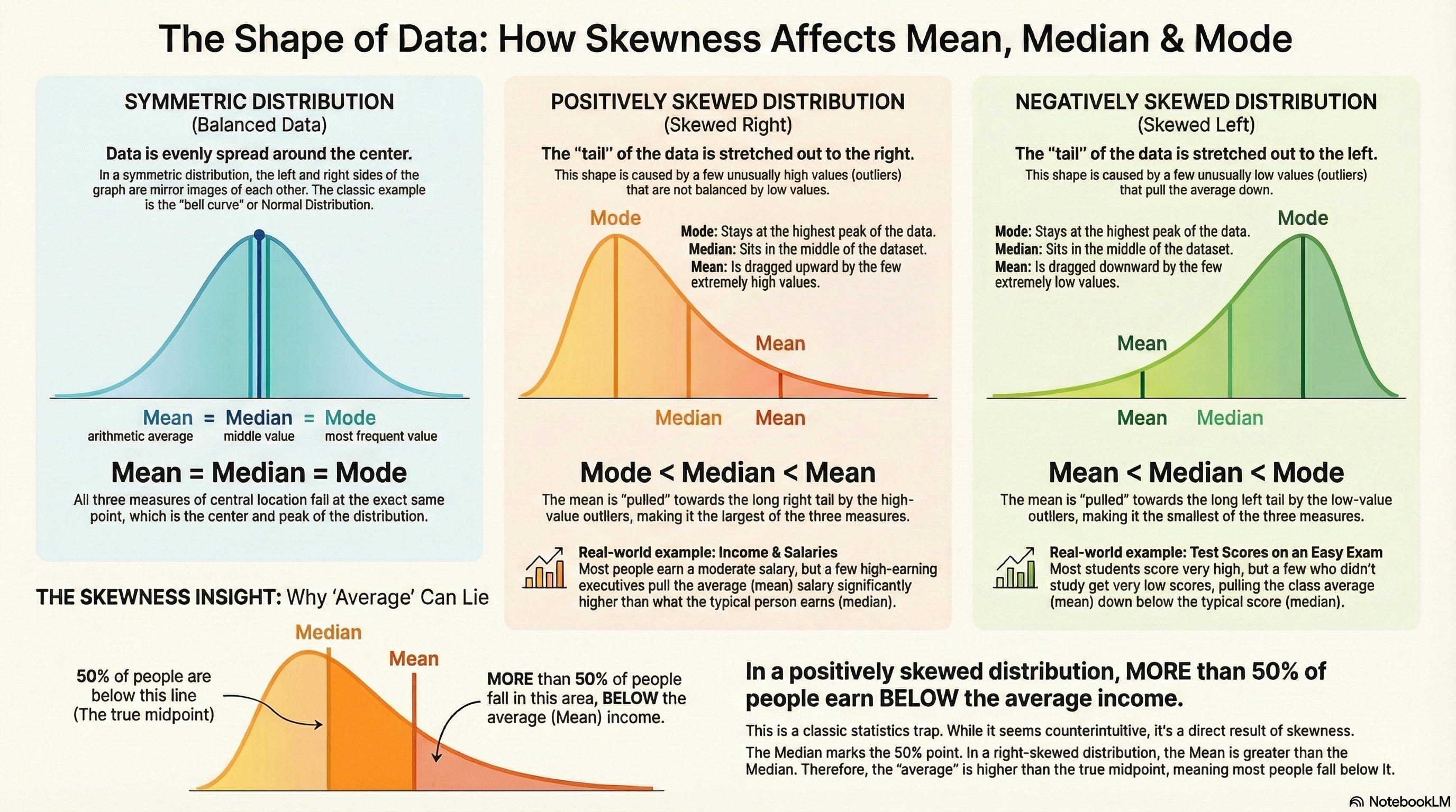
📈 Distribution Shapes & Central Measures

Symmetric Bell-Shaped (Normal Distribution):

        📊
      📊📊📊
    📊📊📊📊📊
  📊📊📊📊📊📊📊
  
Mode = Median = Mean

All three are equal!

---

Symmetric (Two Peaks):

  📊      📊
📊📊    📊📊
📊📊📊📊📊📊

Mode < Median = Mean

Two modes, median and mean still equal

---

Uniform Distribution:

📊📊📊📊📊📊📊

No clear mode
Median = Mean

---

Positive Skew (Right Tail):

📊📊📊
📊📊📊📊
📊📊📊📊📊📊  →

Mode < Median < Mean

Mean pulled by high values!

💡 Memory hack: "Mean follows the tail" - gets pulled toward outliers

Example: Salaries - few very high earners pull mean up

---

Negative Skew (Left Tail):

        📊📊📊
      📊📊📊📊
← 📊📊📊📊📊📊

Mean < Median < Mode

Mean pulled by low values!

---

📋 Decision Guide: Which Measure to Use?

Situation	Best Measure	Why
Symmetric data, no outliers	Mean	Uses all info, most precise
Skewed data	Median	Not affected by extreme values
Categorical data	Mode	Only option!
Need "most typical"	Mode	Most common actual value
Extreme outliers present	Median	Robust against extremes

---

🎯 Test Question Practice

Question: "University graduate salaries are positively skewed. Therefore, the percentage earning above average is greater than the percentage earning below average."

True or False?

Answer: FALSE!

Explanation:

• Positively skewed → tail on right (high salaries)

• Mean gets pulled UP by extreme high salaries

• Mean > Median

• Since median splits data 50-50:

  • 50% earn below median

  • 50% earn above median

• Since mean > median:

  • MORE than 50% earn below mean

  • LESS than 50% earn above mean

💡 Memory hack: In positive skew, the mean "chases" the few rich people, leaving most below average!

---

📊 Advanced Concepts

Skewness

Measures asymmetry of distribution:

$\text{Skewness} = 0 \rightarrow \text{Symmetric}$

$\text{Skewness} > 1 \rightarrow \text{Highly right-skewed}$

$\text{Skewness} < -1 \rightarrow \text{Highly left-skewed}$

Rule of thumb:

• Between -0.5 and 0.5 → Approximately symmetric

• Between 0.5 and 1 (or -0.5 and -1) → Moderately skewed

• Beyond ±1 → Highly skewed

---

Kurtosis

Measures "peakedness" of distribution:

• Mesokurtic (Kurt = 3): Normal distribution

• Leptokurtic (Kurt > 3): Tall and thin peak, heavy tails

• Platykurtic (Kurt < 3): Flat peak, light tails

---

🎓 Key Formulas Summary

Measure	Formula	Use When
Mode	Value with highest f(x) or d	Any variable type
Mean (raw)	$\bar{x} = \frac{\sum x_i}{n}$	Individual data
Mean (frequency)	$\bar{x} = \frac{\sum x_i f_i}{\sum f_i}$	Frequency table
Mean (relative)	$\bar{x} = \sum x_i p_i$	Relative frequency
Median (odd n)	$\tilde{x} = x_{\frac{n+1}{2}}$	Sorted odd data
Median (even n)	$\tilde{x} = \frac{x_{\frac{n}{2}} + x_{\frac{n}{2}+1}}{2}$	Sorted even data
Linear transform	$\bar{z} = a + b\bar{x}$	When transforming all data

---

💡 Master Memory Hacks

1. Sigma ∑ = Smart calculator that adds for you

2. Mode = Most Often Displayed Everywhere

3. Mean = Everyone gets equal share

4. Median = The middleman/bodyguard (protects from extremes)

5. Multiplication & Squares = Cannot split the sum!

6. Mean follows the tail in skewed distributions

7. Midpoint = Average of class limits

8. F(x) = Climbing stairs - keep adding

---

🎯 Quick Reference Mind Map

---

⚠️ Common Exam Mistakes

❌ Splitting multiplication/squares in sigma sums

❌ Using frequency instead of density for continuous mode

❌ Forgetting to sort data before finding median

❌ Confusing "at least" with "at most"

❌ Thinking positive skew means more above average

❌ Using mean when there are extreme outliers

---

🏆 Pro Exam Tips

1. See ∑? Check if you can pull constants out!

2. Finding mode in continuous? Look for highest DENSITY (d), not frequency!

3. Extreme values present? Use median, not mean

4. Positive skew? Mean > Median > Mode (remember: mean follows tail)

5. Linear transformation? Apply it to the measures directly

6. Frequency table? Use weighted formula (x × f)

Remember: The distribution shape tells you the relationship between mode, median, and mean!